Arm Coordinate Frames

• Recall from Lecture 3 that we defined a world coordinate frame (w in the figure below) that is fixed to the environment, with standard basis and origin . The axis of world frame points up from the ground, and we normally draw the axis pointing right and the axis pointing up.
• We also defined a robot frame (r in the figure below) that moves with the robot. It has basis and origin at the point on the ground midway between the two wheel contact points. (The basis and origin vectors of robot frame are expressed in world frame coordinates.) (i.e. the axis of robot frame also points up from the ground), always points directly forward on the robot, and always points to the robot’s left. is the CCW positive angle from to (i.e. from the world frame axis direction to the robot frame axis direction).
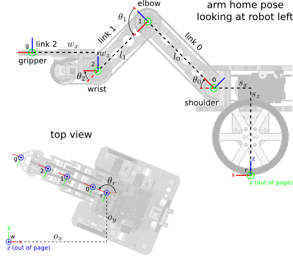
• We now define several coordinate frames on the arm (see figure below):
  • Frame 0 is attached to link 0 on the arm, the initial link that is rotated by the arm shoulder joint. The axis of frame 0 points down link 0; the axis points to robot left, and the axis points “up” on link 0. The origin of frame 0 is the point where the arm shoulder rotation axis intersects the plane of robot frame, which is at the fixed location in robot frame.
  • Frame 1 is attached to link 1 on the arm, the second link that is rotated by the arm elbow joint. The axis of frame 1 points down link 1; the axis points to robot left, and the axis points “up” on link 1. The origin of frame 1 is the point where the arm elbow rotation axis intersects the plane of robot frame, which is at the fixed location in frame 0.
  • Frame 2 is attached to link 2 on the arm, the third link that is rotated by the arm wrist joint. This is also the link that carries the gripper. The axis of frame 2 points down link 2; the axis points to robot left, and the axis points “up” on link 2. The origin of frame 2 is the point where the arm wrist rotation axis intersects the plane of robot frame, which is at the fixed location in frame 1.
  • Frame g (gripper frame) is also attached to link 2; it models the point where an object could be gripped. It is co-oriented with frame 2, and its origin is the center of the circular notch between the gripper fingers, which is at the fixed location in frame 2.
• The arm joint angles are
  : the CCW positive angle from the direction of to
  : the CCW positive angle from the direction of to
  : the CCW positive angle from the direction of to .
• Positive values of each rotate the arm down (i.e. these are right-hand-rule rotations about the corresponding axes).
• The ranges of motion are
  ,
  ,
  , .
• The figure shows the arm in home pose which has , , , and the gripper closed.
• We also define a calibration pose where the arm is pointing straight forward, i.e. and the gripper is closed.

Forward Kinematics

• In Lecture 3 we also developed the forward position kinematics of the robot mobility, including a mathematical function with inputs (the robot pose) and output , a homogenous transformation matrix taking coordinates in robot frame to world frame.
• We can restate this function using two components:
  • is a pure translation transform
  • is a pure rotation about the axis
• Then .
• Remember, transforms compose from right to left. Given a 3D point in robot frame, transform it to world frame by appending an extra 1 and then left-multiply by :
• We now extend this function to include the arm; the inputs will be , and the output will be , a homogenous transformation matrix taking gripper frame to world frame.
• Defining as a pure rotation about the axis, continue the composition to include transforms all the way from gripper frame to world frame:
  
• Using abbreviations and , and observing that the product of a pure translation and a pure rotation (in that order) is given simply by copying the upper left submatrix of the rotation and the upper right submatrix of the translation,
  
  
  
  
  ,
  ,
  
• This shows that the transform taking gripper frame to robot frame is the product of a pure translation and a pure rotation:
  
• In other words,
  • the orientation of the gripper in the robot frame plane is , i.e. the CCW positive angle from to is the sum of the joint angles
  • the gripper location in robot frame (the grip point) is
  • in this case, both of these results could have been found directly using only basic trigonometry
  • but the transform composition formalism with homogenous transformation matrices works the same way for a very broad class of kinematic chains, not just this particular gripper, and it is efficient

Analytic Inverse Kinematics

• Just as inverse position kinematics was very useful for robot mobility, it will also be useful for the arm.
• Conceptually, we would like to literally invert the forward kinematic function.
  • Recall that for robot mobility, this meant finding some drive trajectory that would bring the robot to a desired pose .
  • For the arm, we can define the inverse kinematic problem as finding a set of joint angles that put the gripper at a desired location and orientation in the robot frame plane.
  • Later, we’ll show a simple extension that also uses turn-in-place wheel motions to allow the arm to reach a 3D volume in world frame.
• We’ll also start with one additional simplification: we will only solve a version of the problem where . That is, we will solve a restricted version of the arm IK problem where the gripper is always held parallel to the ground. This simplifies the math somewhat while still demonstrating the essence of IK. Also, it’s not too much of a compromise in many practical grasping tasks. Below we will also show an extension to allow arbitrary .
• Inverse kinematics is a well-studied area. There are a number of approaches; two common ones are analytic (or closed form) IK and numeric (or iterative optimization) IK. We’ll first demonstrate an analytic IK solution for our arm; later we’ll re-solve the problem using the numeric approach.
• The basic idea of analytic IK is to try to algebraically invert the forward kinematics equations. When this is possible (and it is not always possible), the approach has several key properites:
  1. Once the IK equations are found (on paper), they can be coded up, and at runtime their solution(s) can be found (by definition) in constant time. So analytic IK is usually fast.
  2. Note carefully: there can be more than one solution. For example, in our version of the problem, the elbow could “kink” up or down.
  3. Unreachable targets are also identified in constant time.
• Here’s one way to solve our version of the IK problem with an analytic approach:
  • First, since , we can immediately derive
    (1)
    
  • The same fact implies and , which lets us simplify
    
    
    to
    
    
    
  • Now expand the trig identities for angle sums
    (2)
    (3)
    
  • and add the two identities
    (4)
    (5)
    
  • Tecnically (2-5) are a system of 4 equations in 4 unknowns ( ), so we should be able to solve for all unknowns.
  • This is a little tricky unless we apply some geometric insight. Define the reach triangle with vertices given by the origins of frames 0, 1, and 2 (i.e. the intersections of the shoulder, elbow, and wrist rotation axes with the vertical plane in robot frame).
  • TBD diagram
  • Two of the triangle side lengths are and ; the angle between those two sides is . Defining the reach vector in world frame as
    , ,
    the third side has length
    (6)
    
  • Apply the cosine angle difference identity and the law of cosines to solve for :
    (7)
    (8)
    
  • If then (8) implies , but otherwise the given target is unreachable.
  • Assuming the target is reachable, use (5) to find , taking the positive branch of the square root to make the arm “kink up”, i.e. to find a solution with :
    (9)
    
  • Together, (8-9) determine . (10)
    
  • The target is unreachable if , otherwise continue.
  • The final job is to calculate . It will be the difference of the orientation
    (11)
    of the reach vector and the angle in the reach triangle between the sides with lengths and : (12)
    
  • TBD diagram
  • can be found by another application of the law of cosines:
    . (13)
    
  • The target is unreachable if or .
  • Finally, calculate by (1); the target is reachable iff .
  • Summing up: is calculated by (10), which depends on (6,8,9); then is calculated by (12) which depends on (6,11,13); and finally is given by (1).
• This approach can be extended to include a “yaw” rotation by using the wheels to turn in place, which allows the arm to reach a 3D volume in world frame.
  • Let the 3D target location for the gripper be in world frame, and assume that the robot reference point is at the world frame origin
    • if the robot is not at the origin in world frame then subtract the robot location in the world from to get the relative vector from the robot reference point to the gripper target location in world frame
      (14)
      
  • Calculate the yaw angle . (15)
    
  • Transform to with the robot at orientation :
    
  • This boils down to
    ,
    
    
    or (16)
    where is the distance from robot frame origin to the projection of the grip point on the ground plane, and are the coordinates of the grip point in robot frame.
  • TBD diagram
  • Continue as above with the target in the robot frame plane.
  • Summing up:
    1. (first apply (14) to make the grip target relative to the robot location)
    2. apply (15) to get the robot orientation from
    3. apply (16) to get the robot frame grip point from
    4. calculate from (10), from (12), and from (1)
• To extend to arbitrary , not just the special case as developed so far TBD
  • alter the calculation of the reach vector:
  • and use instead of (1)
  • TBD diagram
  • is the absolute CCW-positive tilt angle of the gripper in the robot frame plane

Types of Kinematic Systems

• In general, a kinematic system is composed of links and joints.
  • Links are rigid bodies like our robot’s body and arm segments.
  • Each joint connects two links and allows some kind of relative motion.
  • We will discuss different types of joints below.
• We have now studied two examples of kinematic systems: the mobility system and the arm on our robot.
  • Our robot’s mobility is a planar kinematic system.
  • The arm can either be considered another planar kinematic system, if only the wrist, elbow, and shoulder joints are included, or a spatial kinematic system if the robot’s turn-in-place capability is considered as a fourth “waist” joint.
• For planar kinematic systems link frames are generally described by three degrees of freedom (DoF).
  • That is, the minimum number of scalars needed to completely describe the pose of a link relative to an external world frame is three.
  • For example, our robot’s mobility system controls the pose of the robot base with respect to the world which we parameterize as .
• For spatial kinematic systems link frames are generally described by six DoF.
  • Using both drive and arm motions, the gripper on our robot’s arm can reach any 3D point in a certain range of heights above the ground, giving 3 translational DoF.
  • Two additional rotational DoF can also be independently controlled:
    • the pitch of the gripper, i.e. the angle the plane of the gripper makes with the ground plane.
    • the yaw of the gripper, i.e. the compass direction in which it is pointing (on our robot this will always be the same as the robot heading )
  • Due to the particular construction of our robot the gripper roll angle cannot be controlled. This would be the rotation angle about the link 2 frame axis. That would be the third rotational (and sixth total) DoF.
• In general, the links and joints of a kinematic system form a topological graph, sometimes called the kinematic graph.
• There are various ways to form such a graph, but in one common approach the links are graph vertices and the joints are graph edges.
  • Each link has a coordinate frame that moves rigidly with it.
  • Each joint has a coordinate transform that relates the pose of the two attached link coordinate frames.
• Kinematic graphs are usually connected, i.e. there is a path in the graph from each vertex to every other vertex.
  • Because kinematics is the study of the shape of motion without considering the causes of the motions (physics), kinematics alone cannot say much about the relative motion of disconnected systems.
• Kinematic graph structure is one important way to differentiate classes of kinematic systems.
• The graph of an open chain kinematic system has no loops, i.e. it is a tree.
  • Typically one link is identified as the base of the kinematic system, and is the root of the tree.
  • Tthe leaves of the tree are considered the effectors.
  • Since the graph is a tree, each joint has an unambiguous parent link closer to the base and a child link further from the base.
  • The transform of a joint can be considered to take coordinates from its child link frame to its parent link frame.
  • The pose of any link in an open chain system relative to the base
  • The arm on our robot is an example of one of the simplest (but also most common) types of open chain kinematic systems: an unbranched serial chain.
  • The base of this chain is either the body of the robot, when the joints of the chain are considered to be only the arm wrist, elbow, and shoulder; or if the robot’s turn-in-place capability is considered as a fourth arm joint (the “waist”), the base of the chain is the ground under the robot.
  • The effector of our arm chain is link 2, the link which carries the gripper.
• If the kinematic graph has one or more loops, the system is closed chain.
  • Unlike open chain systems, the kinematic graph alone does not unambiguously identify any particular base or effector links.
  • Whereas for open chain systems it is generally possible to set each joint independently (ignoring self-collisions and collisions with obstacles in the world), for closed chain systems some combinations of joint poses are inadmissable.
  • The forward kinematics of closed chain systems are typically more complex than for open chain systems because of these constraints on the joint angles.
• If the connectivity of the kinematic graph changes on-line the system is structure changing.
  • For example if a robot with two arms can rigidly attach its hands together, it can form a structure changing kinematic system. When the hands are not attached the system is open-chain; when they are attached it is closed-chain.
• The terminology serial/parallel is related to the closed/open chain distinction.
  • However these terms typically refer specifically to systems with one identified base and one effector.
  • Serial systems, like our robot’s arm, connect the base to the effector through intervening links but with no loops in the kinematic graph.
    • Typically up to 3 joints are included for planar serial chains and up to 6 for spatial serial chains, corresponding to the number of relative DoF of the effector to the base in each case.
    • As we will see below, joints typically allow 1 DoF of relative motion each.
    • Though in most cases individual joint DoF do not map directly to the DoF of the effector’s pose — this is why inverse kinematics for serial chains can be nontrivial.
  • Parallel systems connect the base and effector with multiple kinematic chains, forming a closed-chain graph.
    • One class of highly studied parallel kinematic system is the Gough-Stewart platform.

Joint Types

• Joints in a planar kinematic system can theoretically allow up to 3-DoF motion between their attached links, and joints in spatial systems could allow up to 6-DoF of motion.
• However, in practice, most joints allow only one DoF.
  • actuated joints have some type of actuator (like an electric motor) and typically these can only control one DoF at a time.
  • unactuated joints are also possible, but not that common in practice except in parallel robots.
  • It is usually simpler to build accurate one-DoF joints and then chain them together to achieve multiple DoF.
• A revolute joint has one rotational DoF.
• A prismatic joint has one translational DoF.
• These are the two most important joint types. However, there are certainly more.
• For example, a helical joint (like a screw) has one DoF but allows both rotation and translation ; the two are coupled by the joint pitch : .
• One approach to categorize joint types splits those which maintain a surface of contact, called the lower pairs, from other types, called the higher pairs.
  • This terminology originated in the steam age and was developed by people including Franz Reuleaux.
  • The lower pairs are practical joints to build in machinery because high stresses can develop if there is only a point or line of contact vs. an entire continuous area.
• For planar systems the only lower pairs are revolute, prismatic, and planar.
• The possible lower pairs in a spatial system include those three plus helical, spherical, and cylindrical joints.
• TBD diagram.
• It has been proven (TBD ref) that these are the only possible lower pairs.
• Planar and sperhical joints have 3 DoF. Cylindrical joints have 2 DoF. When such multi-DoF joints are implemented in practice they are typically unactuated, e.g. a ball-and-socket assembly is an unactuated spherical joint (with a limited range of motion due to the constraints of attaching to the ball and socket).

Numeric Inverse Kinematics

• Our approach to develop the forward kinematics for our robot arm generalizes fairly easily to the entire class of open-chain systems. The pose of any effector relative to the base can be calculated as
  
  where is the child-to-parent transform of the parent joint of link , is the transform of the next joint on the way to the base, and so on to the last transform of the last joint in the chain which attaches to the base.
• TBD diagram
• Note that this works without modification even for branched systems with multiple end effectors.
• This calculation can defined as the forward kinematic function: the inputs are the joint angles, and the output of the function is the relative pose of the effector to the base:
  
• For planar systems the joint transform function for a revolute joint can be defined as
  
  where is an arbitrary (but fixed by the way the joint is built and assembled to the adjacent link) child-to-mobility transform, and similarly is a mobility-to-parent transform (these can be called positioning transforms).
• For planar systems the joint transform function for a prismatic joint can be defined as
  
• The positioning transforms allow the rotation or translation to effectively work in any direction even though the center mobility transform in the first cse is constructed to only allow rotation about the axis, and in the second case only translation.
• These can easly be exteded to the spatial case using transforms.
• Define the following three functions to extract the -axis rotation and - and -axis translations from a homogenous planar transformation matrix:
  
  
  
  
• For the spatial case it not hard to extend and to 3D and to define , but it is more complex to handle the angle. Spatial rotations have 3 DoF; one option is to generalize to three functions giving the pitch, roll, and yaw of the effector relative to the base. These are sometimes called Euler angles. However, other representations including quaternions and the exponential map Are often used. The full story is interesting but more than we can cover here.
• Then the forward kinematic function can be considered to have inputs and 3 outputs:
  
• The inverse kinematic function would have outputs and 3 inputs:
  
• In general is nonlinear so it can be tricky or impossible to invert analytically, as we did above for the relatively simple arm of our robot.
• An alternative is to numerically approximate the action of using a local linearization, essentially a first-order Taylor approximation:
  
  or in matrix and vector notation
   
  (17)
   
  where and is the Jacobian matrix of at .
• The top row of the Jacobian is a vector that locally approximates as the multiplication of the vector by the vector
• The remaining rows are similar approximations for and
• Another way to understand the Jacobian is by column: each column is a vector of the sensitivities of the EE pose DoF to small movements of joint relative to its starting value
• Define the original EE pose given joint angles as , and the change in EE pose from to a new location at joint angles as .
• Then (17) implies
   
  .
   
  
• Subtract from both sides and multiply by the inverse of the Jacobian, giving
   
  (18)
   
• As long as the Jacobian is in fact invertible (more on this below), this is effectively an incremental solution to the inverse kinematics problem:
  1. Let be the initial joint angles, , and be the goal for the EE pose.
  2. While where is a small tolerance value:
     1. Calculate an updated Jacobain
     2. Let for a small stepsize
     3. Calculate
     4. Update the joint angles:
     5. Update the EE pose:
     6. 
• The Jacobian can only be invertible if it is square, i.e., if the kinematic system has the same number of joints as EE DoF. However, even a square matrix may be noninvertible. Such singular Jacobians arise at specific configurations of the robot, often “outstretched” cases where a robot arm is reaching directly outwards like the calibration pose of our robot. In such configurations small motions in more than one joint yeild infinitesimally equivalent EE motions, and consequently some subspace of EE motions that are normally possible are not reachable. TBD figure.
• Both problems can be worked around, to some extent, by using a pseudoinverse instead of a true inverse. Even better variations on this approach are described in Buss 2009.
• Additional issues that often need to be considered in practice include correct handling of joint motion limits and prioritization of multiple simultaneous goals. See the Buss paper and Baerlocher and Boulic 2004 for useful techniques to address these.

• Home
• Schedule
• Assignments
• References
• Lectures
• Policies
• OHMM Wiki
• Piazza